一.数学基础

1.信息增益：是原始熵和按条件划分后的条件熵的差值。

增益越大，说明熵下降越大，则分类效果越好

2.bootstrap抽样：从原始样本中“有放回地”随机抽取相同大小的样本，重复多次，用这些“重采样样本”来近似总体的分布特性

二.基本概念

1.决策树

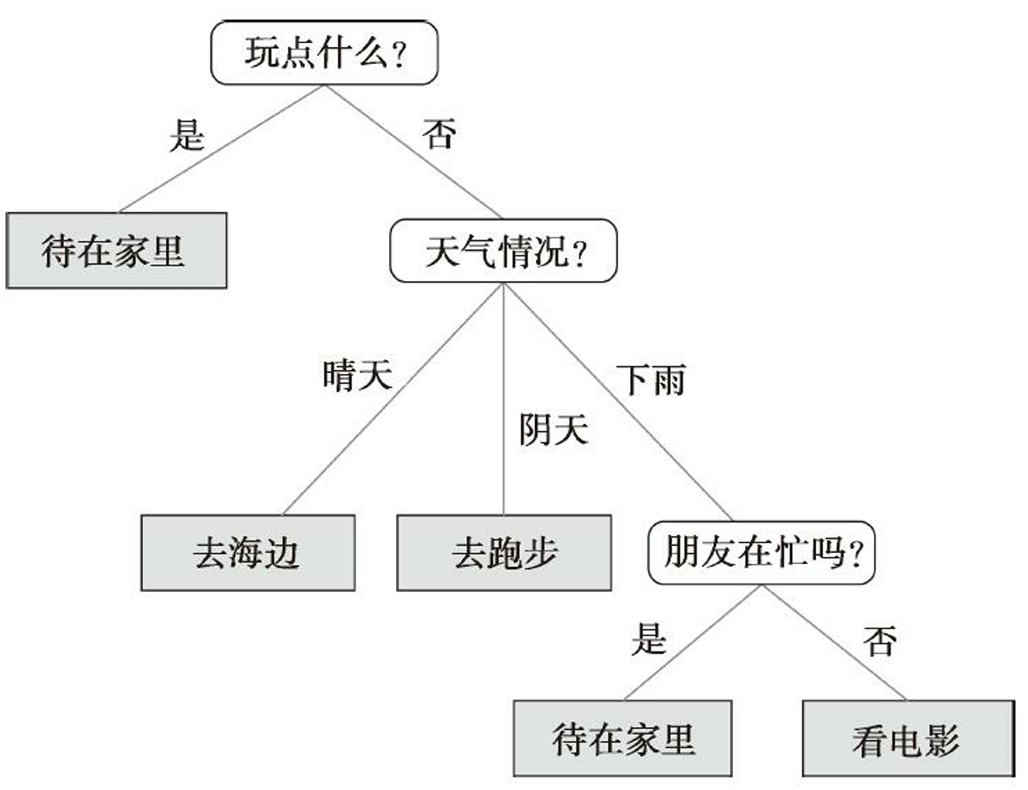
决策树的最大特点是易于解释模型。

二叉决策树的公式为：

D为节点，Dp为父节点，I为不纯度衡量标准，N为样本数量，Np为父节点样本数量

常用的三个不纯度衡量标准为基尼系数、熵和误分类率

熵：

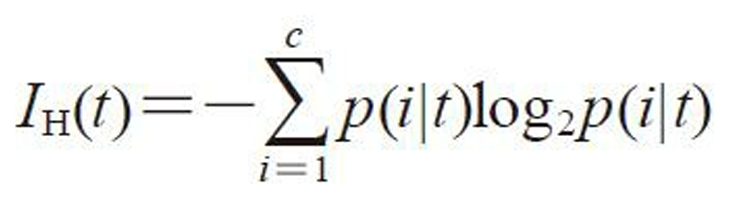
基尼系数，和熵类似，用来评价某个划分对减少不确定性的效果：

误分类率，适用于剪枝阶段：

注：p(i|t)为特定节点t中，属于类别c的样本占特定节点t中样本总数的比例

2.随机森林

即用多个决策树集成来分类，有鲁棒性更强，泛化误差更好，不易过拟合的优点

随机森林的基本步骤为：

a.用bootstrap抽样方法选择n个样本用于训练

b.用步骤a的样本构造一棵决策树，节点划分保证不重复的随机选择d个特征，且根据目标函数的要求（如最大化信息增益），使用选定的特征对节点进行划分

c.重复1~2000次

d.汇总每个决策树的类标进行多数投票

三.scikit-learn库构建决策树

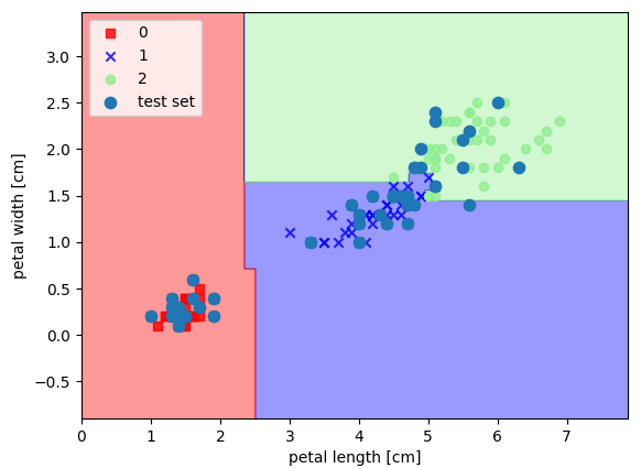
1.决策树

import pandas as pd
from matplotlib.colors import ListedColormap
from sklearn import datasets
from sklearn.model_selection import train_test_split
from sklearn.tree import DecisionTreeClassifier
from sklearn.tree import export_graphviz

iris = datasets.load_iris()
X = iris.data[:, [2, 3]]
y = iris.target
X_train, X_test, y_train, y_test = train_test_split(X, y, test_size=0.3, random_state=0)

sc = StandardScaler()
sc.fit(X_train)
X_combined = np.vstack((X_train, X_test))
y_combined = np.hstack((y_train, y_test))

def plot_decision_regions2(X, y, classifier, test_idx=None, resolution=0.02):
    """
    绘制决策区域
    X: 训练样本
    y: 训练样本的标签
    classifier: 分类器
    test_idx: 测试样本的索引
    resolution: 网格分辨率
    """
    # setup marker generator and color map
    markers = ('s', 'x', 'o', '^', 'v')
    colors = ('red', 'blue', 'lightgreen', 'gray', 'cyan')
    cmap = ListedColormap(colors[:len(np.unique(y))])

    # plot the decision surface
    x1_min, x1_max = X[:, 0].min() - 1, X[:, 0].max() + 1
    x2_min, x2_max = X[:, 1].min() - 1, X[:, 1].max() + 1
    xx1, xx2 = np.meshgrid(np.arange(x1_min, x1_max, resolution),
                           np.arange(x2_min, x2_max, resolution))

    Z = classifier.predict(np.array([xx1.ravel(), xx2.ravel()]).T)
    Z = Z.reshape(xx1.shape)
    plt.contourf(xx1, xx2, Z, alpha=0.4, cmap=cmap)
    plt.xlim(xx1.min(), xx1.max())
    plt.ylim(xx2.min(), xx2.max())

    # plot class samples
    X_test, y_test = X[test_idx, :], y[test_idx]
    for idx, cl in enumerate(np.unique(y)):
        plt.scatter(x=X[y == cl, 0], y=X[y == cl, 1],
                    alpha=0.8, c=cmap(idx),
                    marker=markers[idx], label=cl)

    # highlight test samples
    if test_idx:
        X_test, y_test = X[test_idx, :], y[test_idx]
        plt.scatter(X_test[:, 0], X_test[:, 1], c=None,
                    alpha=1.0, linewidth=1, marker='o',
                    s=55, label='test set')

# 决策树模型
tree = DecisionTreeClassifier(criterion='entropy', max_depth=3, random_state=0)
tree.fit(X_train, y_train)

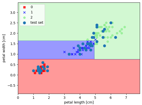
plot_decision_regions2(X_combined, y_combined, classifier=tree, test_idx=range(105, 150))
plt.xlabel('petal length [cm]')
plt.ylabel('petal width [cm]')
plt.legend(loc='upper left')
plt.show()
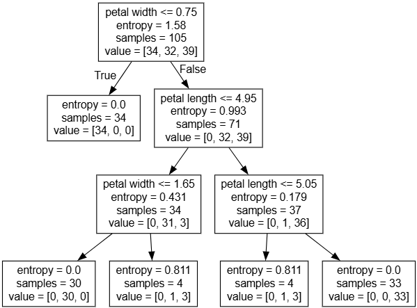
# 导出决策树，可以用vscode的插件Graphviz Interactive Preview或下载graphviz查看
export_graphviz(tree, out_file='tree.dot', feature_names=['petal length', 'petal width'])

2.随机森林

import pandas as pd
from matplotlib.colors import ListedColormap
from sklearn import datasets
from sklearn.model_selection import train_test_split
from sklearn.tree import DecisionTreeClassifier
from sklearn.tree import export_graphviz

iris = datasets.load_iris()
X = iris.data[:, [2, 3]]
y = iris.target
X_train, X_test, y_train, y_test = train_test_split(X, y, test_size=0.3, random_state=0)

sc = StandardScaler()
sc.fit(X_train)
X_combined = np.vstack((X_train, X_test))
y_combined = np.hstack((y_train, y_test))

def plot_decision_regions2(X, y, classifier, test_idx=None, resolution=0.02):
    """
    绘制决策区域
    X: 训练样本
    y: 训练样本的标签
    classifier: 分类器
    test_idx: 测试样本的索引
    resolution: 网格分辨率
    """
    # setup marker generator and color map
    markers = ('s', 'x', 'o', '^', 'v')
    colors = ('red', 'blue', 'lightgreen', 'gray', 'cyan')
    cmap = ListedColormap(colors[:len(np.unique(y))])

    # plot the decision surface
    x1_min, x1_max = X[:, 0].min() - 1, X[:, 0].max() + 1
    x2_min, x2_max = X[:, 1].min() - 1, X[:, 1].max() + 1
    xx1, xx2 = np.meshgrid(np.arange(x1_min, x1_max, resolution),
                           np.arange(x2_min, x2_max, resolution))

    Z = classifier.predict(np.array([xx1.ravel(), xx2.ravel()]).T)
    Z = Z.reshape(xx1.shape)
    plt.contourf(xx1, xx2, Z, alpha=0.4, cmap=cmap)
    plt.xlim(xx1.min(), xx1.max())
    plt.ylim(xx2.min(), xx2.max())

    # plot class samples
    X_test, y_test = X[test_idx, :], y[test_idx]
    for idx, cl in enumerate(np.unique(y)):
        plt.scatter(x=X[y == cl, 0], y=X[y == cl, 1],
                    alpha=0.8, c=cmap(idx),
                    marker=markers[idx], label=cl)

    # highlight test samples
    if test_idx:
        X_test, y_test = X[test_idx, :], y[test_idx]
        plt.scatter(X_test[:, 0], X_test[:, 1], c=None,
                    alpha=1.0, linewidth=1, marker='o',
                    s=55, label='test set')

# 随机森林模型
# n_estimators是森林中树的数量，n_jobs是并行计算任务数量的参数
forest = RandomForestClassifier(criterion='entropy', n_estimators=10, random_state=1, n_jobs=2)
forest.fit(X_train, y_train)
plot_decision_regions2(X_combined, y_combined, classifier=forest, test_idx=range(105, 150))
plt.xlabel('petal length [cm]')
plt.ylabel('petal width [cm]')
plt.legend(loc='upper left')
plt.show()