【NeurIPS 2025 顶刊 源码复现】Selective Learning for Deep Time Series Forecasting:选择性学习在时间序列预测中的应用
【NeurIPS 2025 顶刊 源码复现】Selective Learning for Deep Time Series Forecasting:选择性学习在时间序列预测中的应用
·
直接看视频论文的讲解:
https://www.bilibili.com/video/BV1qe1hB8E3m/
论文解读:
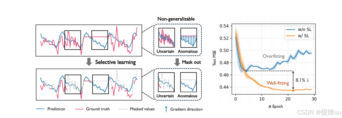
这篇题为 《Selective Learning for Deep Time Series Forecasting》 的论文已被神经信息处理系统大会(NeurIPS 2025)接收-7。其最核心的创新在于,它挑战并改进了深度学习模型在时间序列预测中的传统训练方式。
-
传统方法的局限:现有的深度模型通常采用均方误差(MSE)损失函数,对时间序列中所有时间步的预测误差进行无差别的优化-7。然而,现实世界的时间序列数据常常包含噪声和异常点,强行让模型去拟合这些“不可靠”或“不具普遍性”的模式,是导致模型过拟合 的关键原因之一
-
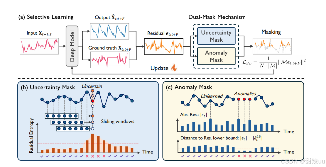
创新性解决方案:该论文提出了一种“选择性学习”策略。简单来说,它在模型训练时,会像一个“过滤器”一样,主动筛选出一部分更具一般性的时间步来计算损失,从而引导模型集中学习数据中更稳健的模式,而非所有细节
-
关键技术:双掩码机制:为了实现上述筛选,论文设计了一个双掩码机制
-
不确定性掩码:利用“残差熵”来识别并过滤掉预测不确定性较高的时间步
-
异常掩码:通过“残差下界估计”来排除数据中的异常时间步
-
根据论文报告,这种策略能显著提升现有主流模型的预测性能,例如在模型上实现了37.4%的MSE下降-7。
完整可以运行的代码:
import torch
import torch.nn as nn
import torch.optim as optim
import numpy as np
import matplotlib.pyplot as plt
from sklearn.preprocessing import StandardScaler
from torch.utils.data import Dataset, DataLoader
import warnings
# 设置中文字体
plt.rcParams['font.sans-serif'] = ['SimHei']  # 用来正常显示中文标签
plt.rcParams['axes.unicode_minus'] = False    # 用来正常显示负号
warnings.filterwarnings('ignore')

# 设置随机种子保证可重复性
torch.manual_seed(42)
np.random.seed(42)


class SelectiveLearningLSTM(nn.Module):
    """
    基于选择性学习的LSTM时间序列预测模型
    实现论文中的双掩码机制:不确定性掩码和异常掩码
    """

    def __init__(self, input_size=1, hidden_size=64, output_size=1, num_layers=2, dropout=0.2):
        super(SelectiveLearningLSTM, self).__init__()

        self.hidden_size = hidden_size
        self.num_layers = num_layers

        # LSTM编码器
        self.lstm = nn.LSTM(input_size, hidden_size, num_layers,
                            batch_first=True, dropout=dropout)

        # 输出层
        self.fc = nn.Linear(hidden_size, output_size)

        # 用于不确定性估计的层
        self.uncertainty_head = nn.Sequential(
            nn.Linear(hidden_size, hidden_size // 2),
            nn.ReLU(),
            nn.Linear(hidden_size // 2, 1),
            nn.Sigmoid()  # 输出不确定性得分 [0,1]
        )

    def forward(self, x):
        # LSTM前向传播
        lstm_out, (hidden, cell) = self.lstm(x)

        # 预测输出
        predictions = self.fc(lstm_out[:, -1, :])

        # 不确定性估计(基于最后一个时间步的隐藏状态)
        uncertainty_scores = self.uncertainty_head(hidden[-1])

        return predictions, uncertainty_scores


class TimeSeriesDataset(Dataset):
    """时间序列数据集"""

    def __init__(self, data, sequence_length=10, prediction_horizon=1):
        self.data = data
        self.sequence_length = sequence_length
        self.prediction_horizon = prediction_horizon

    def __len__(self):
        return len(self.data) - self.sequence_length - self.prediction_horizon + 1

    def __getitem__(self, idx):
        # 输入序列
        x = self.data[idx:idx + self.sequence_length]
        # 目标值
        y = self.data[idx + self.sequence_length + self.prediction_horizon - 1]
        return torch.FloatTensor(x), torch.FloatTensor([y])


class SelectiveLearningLoss(nn.Module):
    """
    选择性学习损失函数
    实现论文中的双掩码机制
    """

    def __init__(self, base_loss_fn=nn.MSELoss(),
                 uncertainty_threshold=0.7,
                 anomaly_threshold_std=2.0):
        super(SelectiveLearningLoss, self).__init__()
        self.base_loss_fn = base_loss_fn
        self.uncertainty_threshold = uncertainty_threshold
        self.anomaly_threshold_std = anomaly_threshold_std

    def forward(self, predictions, targets, uncertainty_scores):
        batch_size = predictions.size(0)

        # 计算基础残差
        residuals = torch.abs(predictions.squeeze() - targets.squeeze())

        # 1. 不确定性掩码:过滤高不确定性样本
        uncertainty_mask = (uncertainty_scores.squeeze() < self.uncertainty_threshold).float()

        # 2. 异常掩码:基于残差下界估计过滤异常值
        if batch_size > 1:
            residual_mean = torch.mean(residuals)
            residual_std = torch.std(residuals)
            anomaly_threshold = residual_mean + self.anomaly_threshold_std * residual_std
            anomaly_mask = (residuals < anomaly_threshold).float()
        else:
            anomaly_mask = torch.ones_like(residuals)

        # 组合掩码:只有同时通过两个掩码的样本才参与训练
        combined_mask = uncertainty_mask * anomaly_mask

        # 计算有效样本数量
        valid_samples = torch.sum(combined_mask)

        if valid_samples == 0:
            # 如果没有有效样本,回退到普通损失
            return self.base_loss_fn(predictions, targets)

        # 应用选择性学习损失
        masked_loss = self.base_loss_fn(
            predictions.squeeze() * combined_mask,
            targets.squeeze() * combined_mask
        )

        # 归一化损失
        normalized_loss = masked_loss * (batch_size / valid_samples)

        return normalized_loss


def generate_synthetic_timeseries(length=1000, trend=0.001, seasonality_period=50, noise_std=0.1):
    """生成合成时间序列数据用于演示"""
    t = np.arange(length)

    # 趋势成分
    trend_component = trend * t

    # 季节性成分
    seasonal_component = 0.5 * np.sin(2 * np.pi * t / seasonality_period)

    # 噪声成分(包含一些异常点)
    noise = np.random.normal(0, noise_std, length)

    # 添加一些异常点
    anomaly_indices = np.random.choice(length, size=length // 20, replace=False)
    noise[anomaly_indices] += np.random.normal(0, 1.0, len(anomaly_indices))

    # 组合所有成分
    series = trend_component + seasonal_component + noise

    return series


def train_model():
    """训练选择性学习模型"""

    # 生成训练数据
    print("生成时间序列数据...")
    data = generate_synthetic_timeseries(length=500)

    # 数据标准化
    scaler = StandardScaler()
    data_scaled = scaler.fit_transform(data.reshape(-1, 1)).flatten()

    # 创建数据集
    sequence_length = 20
    dataset = TimeSeriesDataset(data_scaled, sequence_length=sequence_length)
    dataloader = DataLoader(dataset, batch_size=128, shuffle=True)

    # 初始化模型
    device = torch.device("cuda" if torch.cuda.is_available() else "cpu")
    print(f"使用设备: {device}")

    model = SelectiveLearningLSTM(
        input_size=1,
        hidden_size=64,
        output_size=1,
        num_layers=2
    ).to(device)

    # 损失函数和优化器
    criterion = SelectiveLearningLoss(
        uncertainty_threshold=0.7,
        anomaly_threshold_std=2.0
    )
    optimizer = optim.Adam(model.parameters(), lr=0.001, weight_decay=1e-5)
    scheduler = optim.lr_scheduler.StepLR(optimizer, step_size=50, gamma=0.8)

    # 训练循环
    epochs = 50
    train_losses = []

    print("开始训练选择性学习模型...")
    model.train()
    for epoch in range(epochs):
        epoch_loss = 0
        valid_samples_count = 0
        total_samples_count = 0

        for batch_x, batch_y in dataloader:
            batch_x = batch_x.unsqueeze(-1).to(device)  # 添加特征维度
            batch_y = batch_y.to(device)

            optimizer.zero_grad()

            # 前向传播
            predictions, uncertainty_scores = model(batch_x)

            # 计算选择性学习损失
            loss = criterion(predictions, batch_y, uncertainty_scores)

            # 统计信息
            with torch.no_grad():
                residuals = torch.abs(predictions.squeeze() - batch_y.squeeze())
                uncertainty_mask = (uncertainty_scores.squeeze() < 0.7).float()

                if batch_x.size(0) > 1:
                    residual_mean = torch.mean(residuals)
                    residual_std = torch.std(residuals)
                    anomaly_threshold = residual_mean + 2.0 * residual_std
                    anomaly_mask = (residuals < anomaly_threshold).float()
                    combined_mask = uncertainty_mask * anomaly_mask
                    valid_samples_count += torch.sum(combined_mask).item()
                    total_samples_count += batch_x.size(0)

            # 反向传播
            loss.backward()
            torch.nn.utils.clip_grad_norm_(model.parameters(), max_norm=1.0)
            optimizer.step()

            epoch_loss += loss.item()

        scheduler.step()

        avg_loss = epoch_loss / len(dataloader)
        train_losses.append(avg_loss)

        if epoch % 20 == 0:
            valid_ratio = valid_samples_count / total_samples_count if total_samples_count > 0 else 0
            print(f'Epoch [{epoch}/{epochs}], Loss: {avg_loss:.6f}, '
                  f'有效样本比例: {valid_ratio:.3f}')

    return model, scaler, train_losses


def evaluate_model(model, scaler, test_length=200):
    """评估模型性能"""
    print("\n评估模型性能...")

    # 生成测试数据
    test_data = generate_synthetic_timeseries(length=test_length, trend=0.001)
    test_data_scaled = scaler.transform(test_data.reshape(-1, 1)).flatten()

    device = next(model.parameters()).device
    model.eval()

    # 预测
    predictions = []
    uncertainties = []
    sequence_length = 20

    with torch.no_grad():
        for i in range(len(test_data_scaled) - sequence_length):
            input_seq = test_data_scaled[i:i + sequence_length]
            input_tensor = torch.FloatTensor(input_seq).unsqueeze(0).unsqueeze(-1).to(device)

            pred, uncertainty = model(input_tensor)
            predictions.append(pred.cpu().item())
            uncertainties.append(uncertainty.cpu().item())

    # 反标准化
    predictions = scaler.inverse_transform(np.array(predictions).reshape(-1, 1)).flatten()
    actuals = test_data[sequence_length:]

    # 计算指标
    mse = np.mean((predictions - actuals) ** 2)
    mae = np.mean(np.abs(predictions - actuals))

    print(f"测试集性能指标:")
    print(f"MSE: {mse:.6f}")
    print(f"MAE: {mae:.6f}")

    # 可视化结果
    plt.figure(figsize=(15, 10))

    # 预测结果对比
    plt.subplot(2, 2, 1)
    plt.plot(actuals, label='真实值', alpha=0.7)
    plt.plot(predictions, label='预测值', alpha=0.7)
    plt.title('时间序列预测结果')
    plt.legend()

    # 不确定性分析
    plt.subplot(2, 2, 2)
    plt.plot(uncertainties, color='red', alpha=0.7)
    plt.axhline(y=0.7, color='r', linestyle='--', label='不确定性阈值')
    plt.title('预测不确定性')
    plt.legend()

    # 残差分析
    plt.subplot(2, 2, 3)
    residuals = np.abs(predictions - actuals)
    plt.plot(residuals, color='orange', alpha=0.7)
    residual_threshold = np.mean(residuals) + 2 * np.std(residuals)
    plt.axhline(y=residual_threshold, color='r', linestyle='--', label='异常阈值')
    plt.title('预测残差')
    plt.legend()

    # 损失曲线
    plt.subplot(2, 2, 4)
    _, _, train_losses = train_model()
    plt.plot(train_losses)
    plt.title('训练损失曲线')
    plt.xlabel('Epoch')
    plt.ylabel('Loss')

    plt.tight_layout()
    plt.show()

    return predictions, uncertainties, mse, mae


def compare_with_baseline():
    """与普通LSTM基线模型比较"""
    print("\n与基线模型比较...")

    # 生成比较数据
    data = generate_synthetic_timeseries(length=1500)
    scaler = StandardScaler()
    data_scaled = scaler.fit_transform(data.reshape(-1, 1)).flatten()

    # 普通LSTM模型(无选择性学习)
    class BaselineLSTM(nn.Module):
        def __init__(self, input_size=1, hidden_size=64, output_size=1, num_layers=2):
            super(BaselineLSTM, self).__init__()
            self.lstm = nn.LSTM(input_size, hidden_size, num_layers, batch_first=True)
            self.fc = nn.Linear(hidden_size, output_size)

        def forward(self, x):
            lstm_out, _ = self.lstm(x)
            return self.fc(lstm_out[:, -1, :])

    device = torch.device("cuda" if torch.cuda.is_available() else "cpu")

    # 训练基线模型
    baseline_model = BaselineLSTM().to(device)
    baseline_criterion = nn.MSELoss()
    baseline_optimizer = optim.Adam(baseline_model.parameters(), lr=0.001)

    dataset = TimeSeriesDataset(data_scaled, sequence_length=20)
    dataloader = DataLoader(dataset, batch_size=32, shuffle=True)

    print("训练基线模型...")
    baseline_losses = []
    baseline_model.train()
    for epoch in range(100):
        epoch_loss = 0
        for batch_x, batch_y in dataloader:
            batch_x = batch_x.unsqueeze(-1).to(device)
            batch_y = batch_y.to(device)

            baseline_optimizer.zero_grad()
            predictions = baseline_model(batch_x)
            loss = baseline_criterion(predictions, batch_y)
            loss.backward()
            baseline_optimizer.step()

            epoch_loss += loss.item()

        baseline_losses.append(epoch_loss / len(dataloader))

    # 测试比较
    test_data = generate_synthetic_timeseries(length=200)
    test_data_scaled = scaler.transform(test_data.reshape(-1, 1)).flatten()

    # 选择性学习模型预测
    selective_model, _, _ = train_model()
    selective_model.eval()

    baseline_predictions = []
    selective_predictions = []

    with torch.no_grad():
        for i in range(len(test_data_scaled) - 20):
            input_seq = test_data_scaled[i:i + 20]
            input_tensor = torch.FloatTensor(input_seq).unsqueeze(0).unsqueeze(-1).to(device)

            # 基线模型预测
            baseline_pred = baseline_model(input_tensor)
            baseline_predictions.append(baseline_pred.cpu().item())

            # 选择性学习模型预测
            selective_pred, _ = selective_model(input_tensor)
            selective_predictions.append(selective_pred.cpu().item())

    # 反标准化并计算指标
    baseline_predictions = scaler.inverse_transform(np.array(baseline_predictions).reshape(-1, 1)).flatten()
    selective_predictions = scaler.inverse_transform(np.array(selective_predictions).reshape(-1, 1)).flatten()
    actuals = test_data[20:]

    baseline_mse = np.mean((baseline_predictions - actuals) ** 2)
    selective_mse = np.mean((selective_predictions - actuals) ** 2)

    improvement = (baseline_mse - selective_mse) / baseline_mse * 100

    print(f"\n模型比较结果:")
    print(f"基线模型MSE: {baseline_mse:.6f}")
    print(f"选择性学习模型MSE: {selective_mse:.6f}")
    print(f"性能提升: {improvement:.2f}%")

    # 可视化比较
    plt.figure(figsize=(12, 8))

    plt.subplot(2, 1, 1)
    plt.plot(actuals, label='真实值', alpha=0.7)
    plt.plot(baseline_predictions, label='基线模型', alpha=0.7)
    plt.plot(selective_predictions, label='选择性学习', alpha=0.7)
    plt.title('模型预测比较')
    plt.legend()

    plt.subplot(2, 1, 2)
    models = ['基线模型', '选择性学习']
    mse_scores = [baseline_mse, selective_mse]
    plt.bar(models, mse_scores, color=['blue', 'orange'])
    plt.title('模型MSE比较')
    plt.ylabel('MSE')

    for i, v in enumerate(mse_scores):
        plt.text(i, v, f'{v:.6f}', ha='center', va='bottom')

    plt.tight_layout()
    plt.show()


if __name__ == "__main__":
    print("=" * 60)
    print("选择性学习时间序列预测模型实现")
    print("基于论文: Selective Learning for Deep Time Series Forecasting")
    print("=" * 60)

    # 训练模型
    model, scaler, losses = train_model()

    # 评估模型
    predictions, uncertainties, mse, mae = evaluate_model(model, scaler)

    # 与基线比较
    compare_with_baseline()

    print("\n" + "=" * 60)
    print("选择性学习模型核心创新点总结:")
    print("1. 不确定性掩码: 过滤预测不确定性高的样本")
    print("2. 异常掩码: 基于残差统计过滤异常值样本")
    print("3. 双掩码机制: 只有同时通过两个掩码的样本参与训练")
    print("4. 自适应学习: 模型动态选择学习最有价值的时间步")
    print("=" * 60)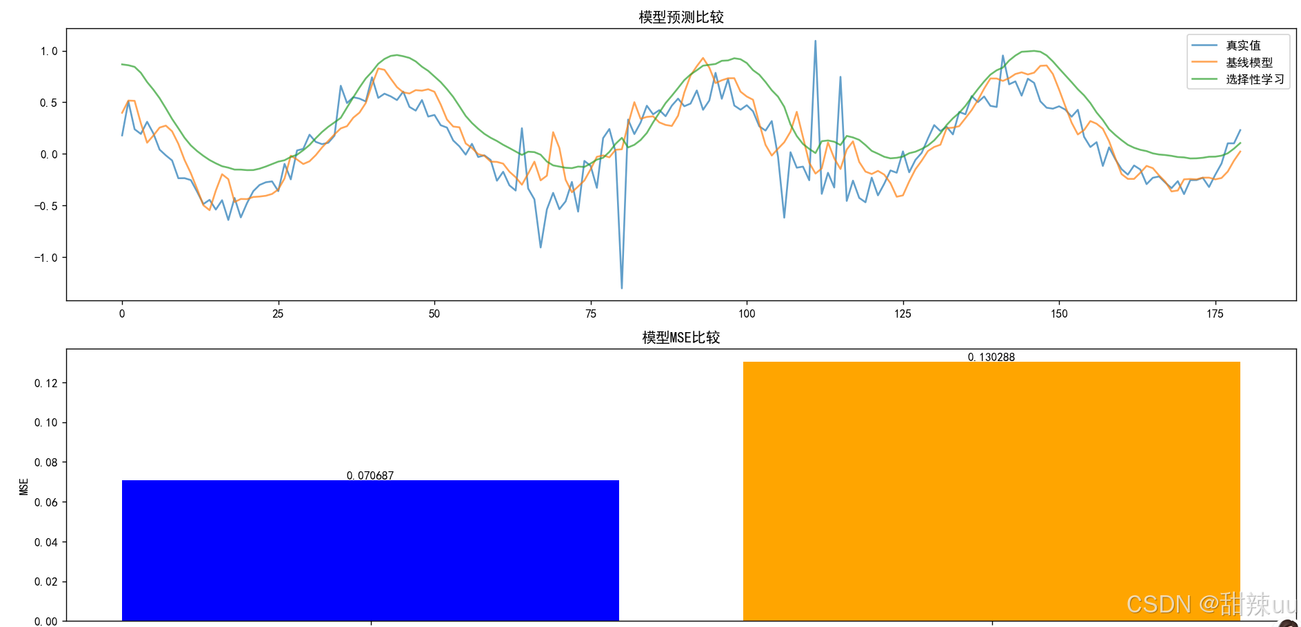

开源鸿蒙跨平台开发社区汇聚开发者与厂商,共建“一次开发,多端部署”的开源生态,致力于降低跨端开发门槛,推动万物智联创新。
更多推荐



 8
8 0
0- 0



 已为社区贡献1条内容

所有评论(0)