使用 Wine 数据集进行朴素贝叶斯分类

学习目标

通过本课程，你将了解到如何使用Python的scikit-learn库进行朴素贝叶斯分类并评估模型性能。

相关知识点

• 贝叶斯分类

学习内容

1 贝叶斯分类

在本课程中，我们将展示如何使用 Python 的 scikit-learn 库中的朴素贝叶斯方法，根据葡萄酒的理化分析数据来分类其产地。这些数据来自意大利同一地区种植但源自三种不同葡萄品种的葡萄酒的化学分析结果。分析确定了每种类型的葡萄酒中 13种成分的含量。

1.1导入包和数据集

import numpy as np
import pandas as pd
import matplotlib.pyplot as plt

%matplotlib inline

1.2读取数据并进行数据分析

数据设置

!wget https://model-community-picture.obs.cn-north-4.myhuaweicloud.com/ascend-zone/notebook_datasets/ab1f8f1eda2011efa1e7fa163edcddae/wine.zip
!unzip wine.zip

df = pd.read_csv('wine.data')
df.head(10)

特征的基本统计信息

df.iloc[:,1:].describe()

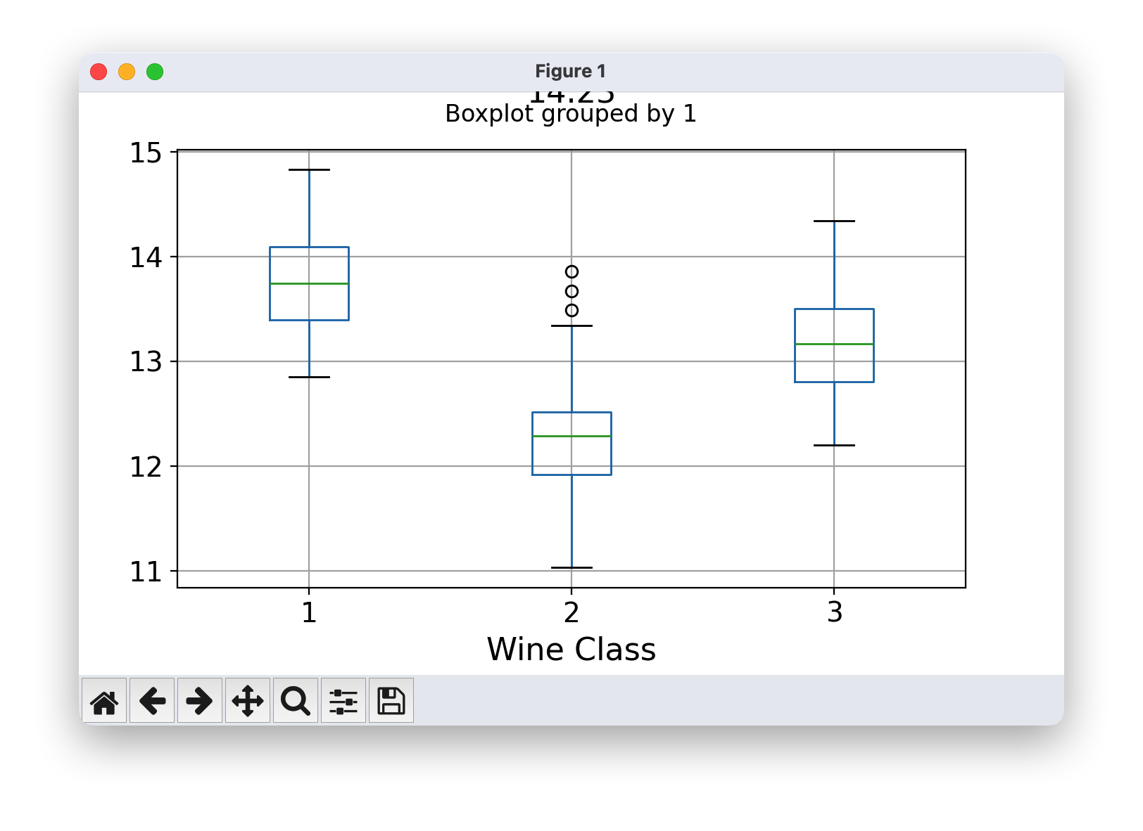
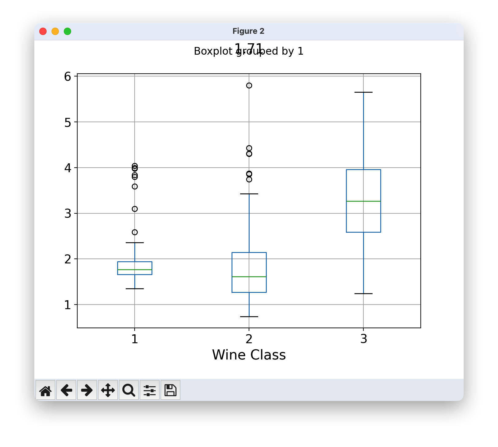
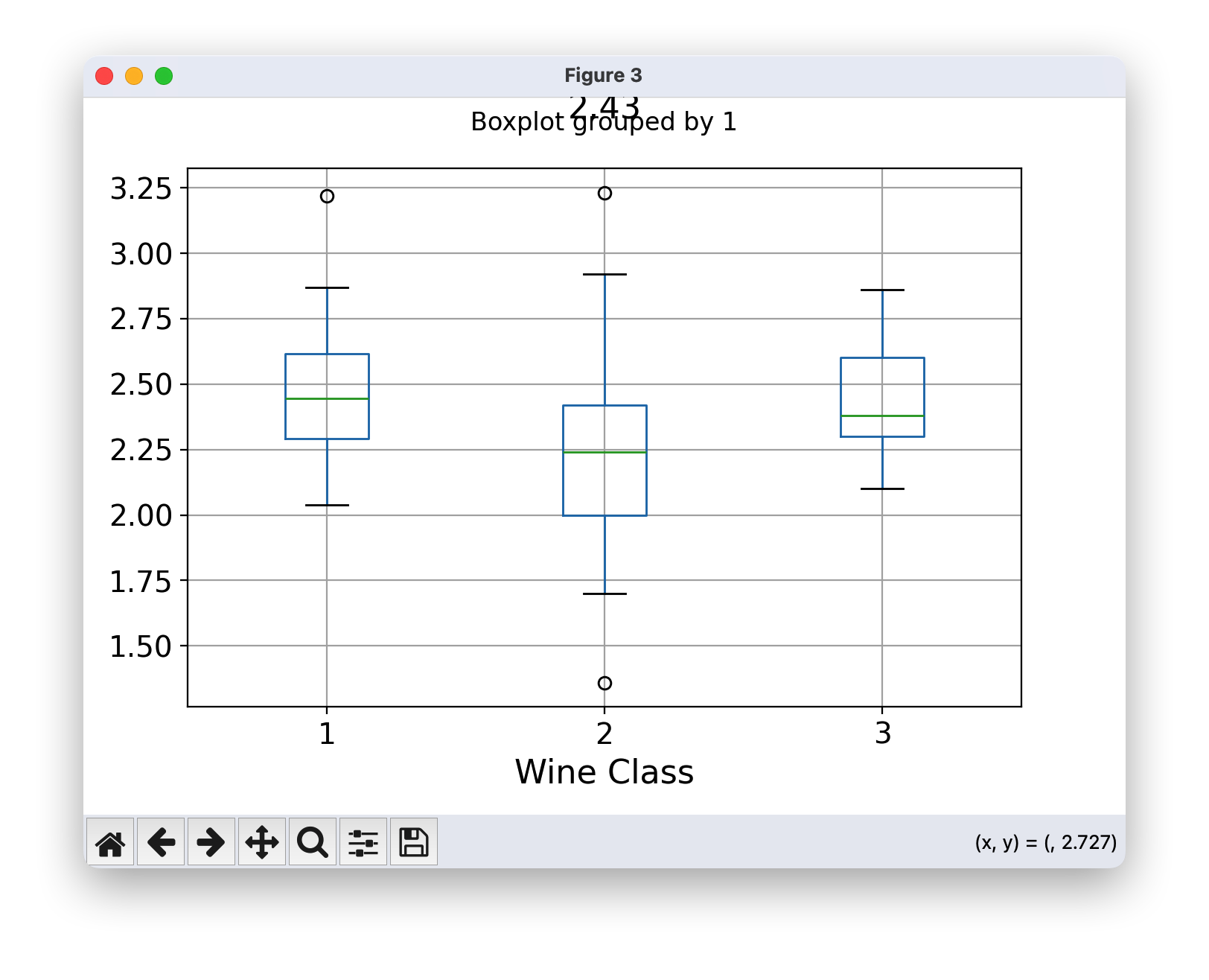
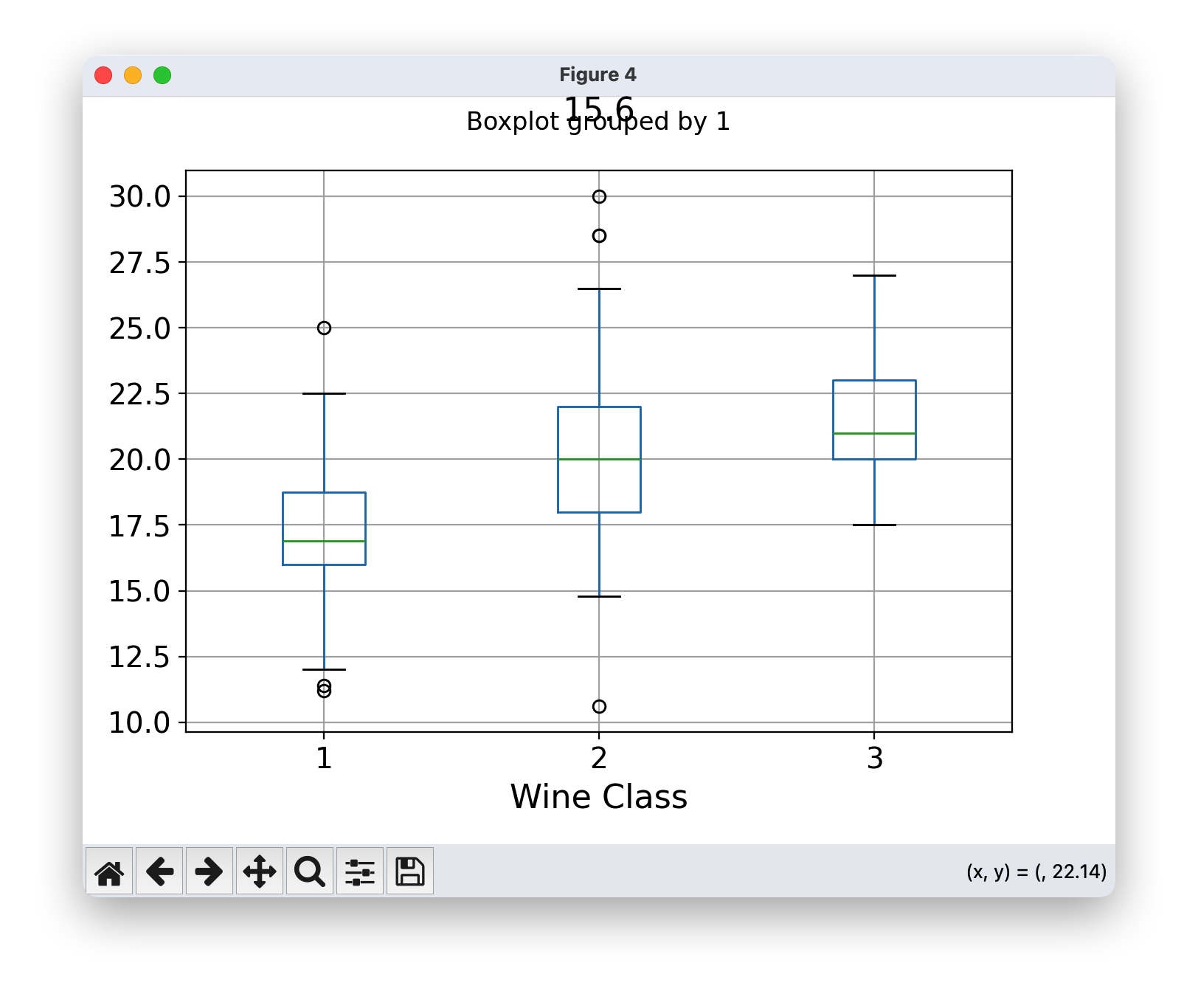
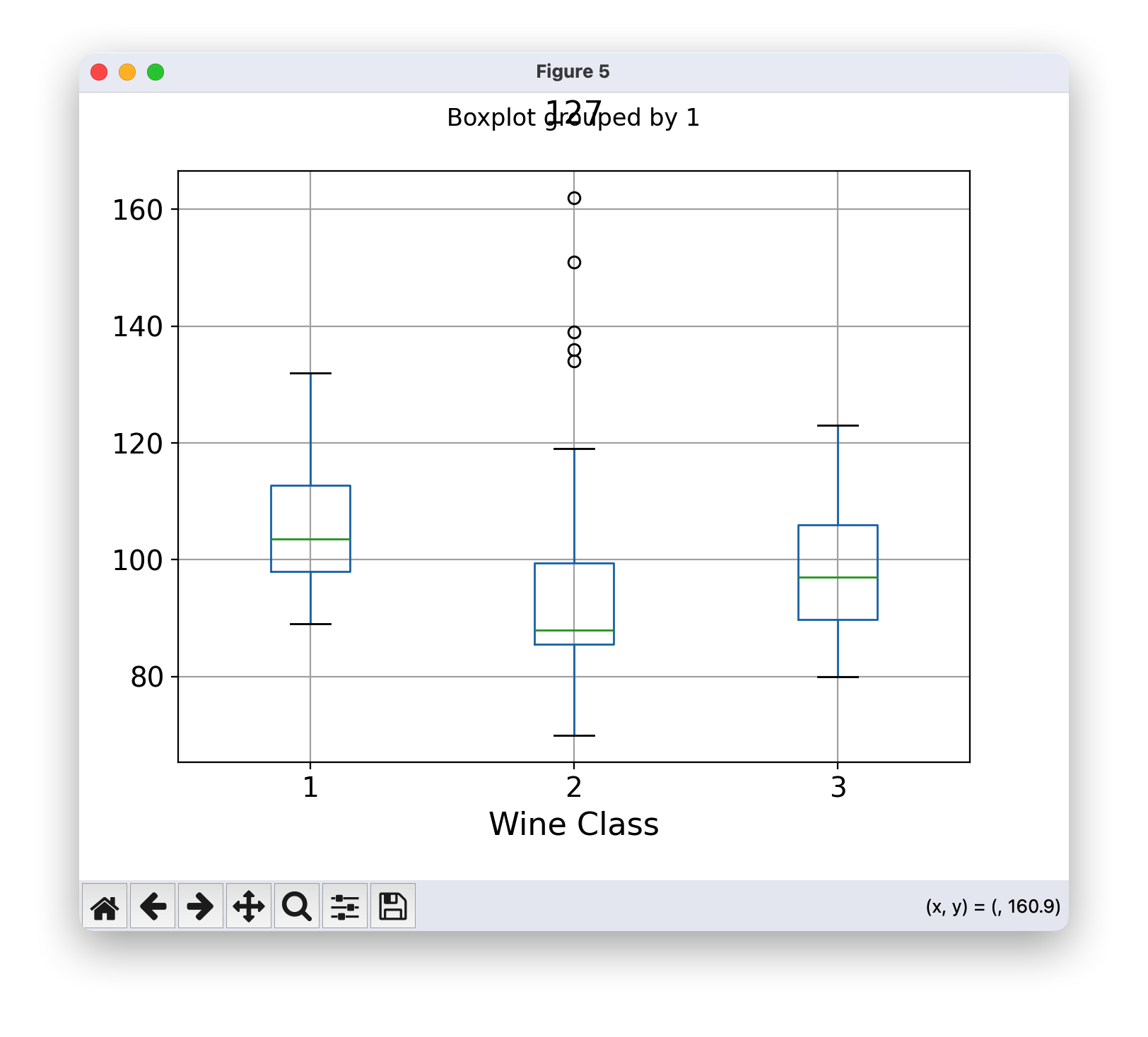
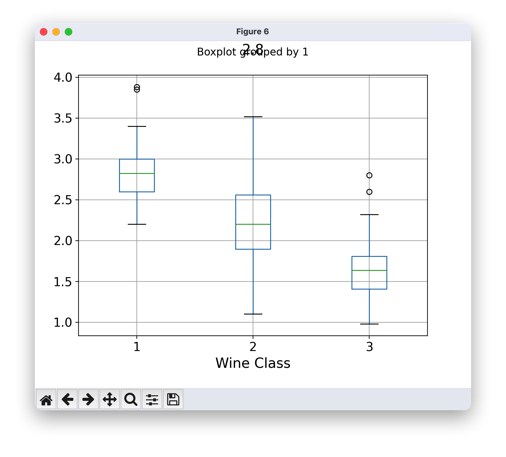
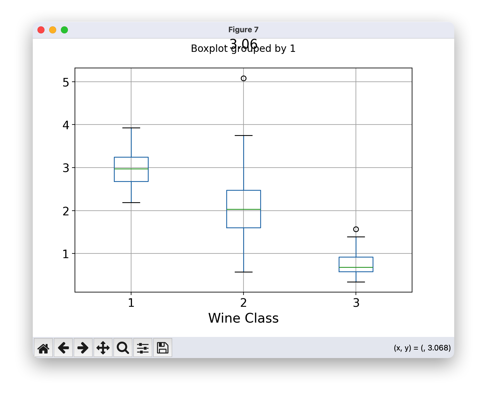
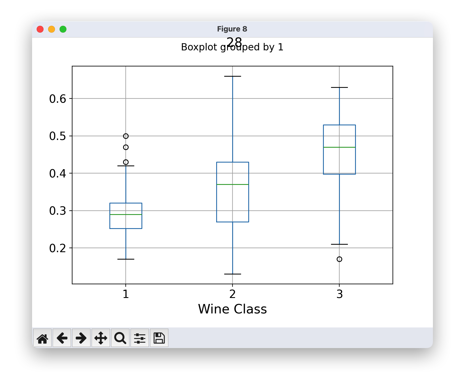
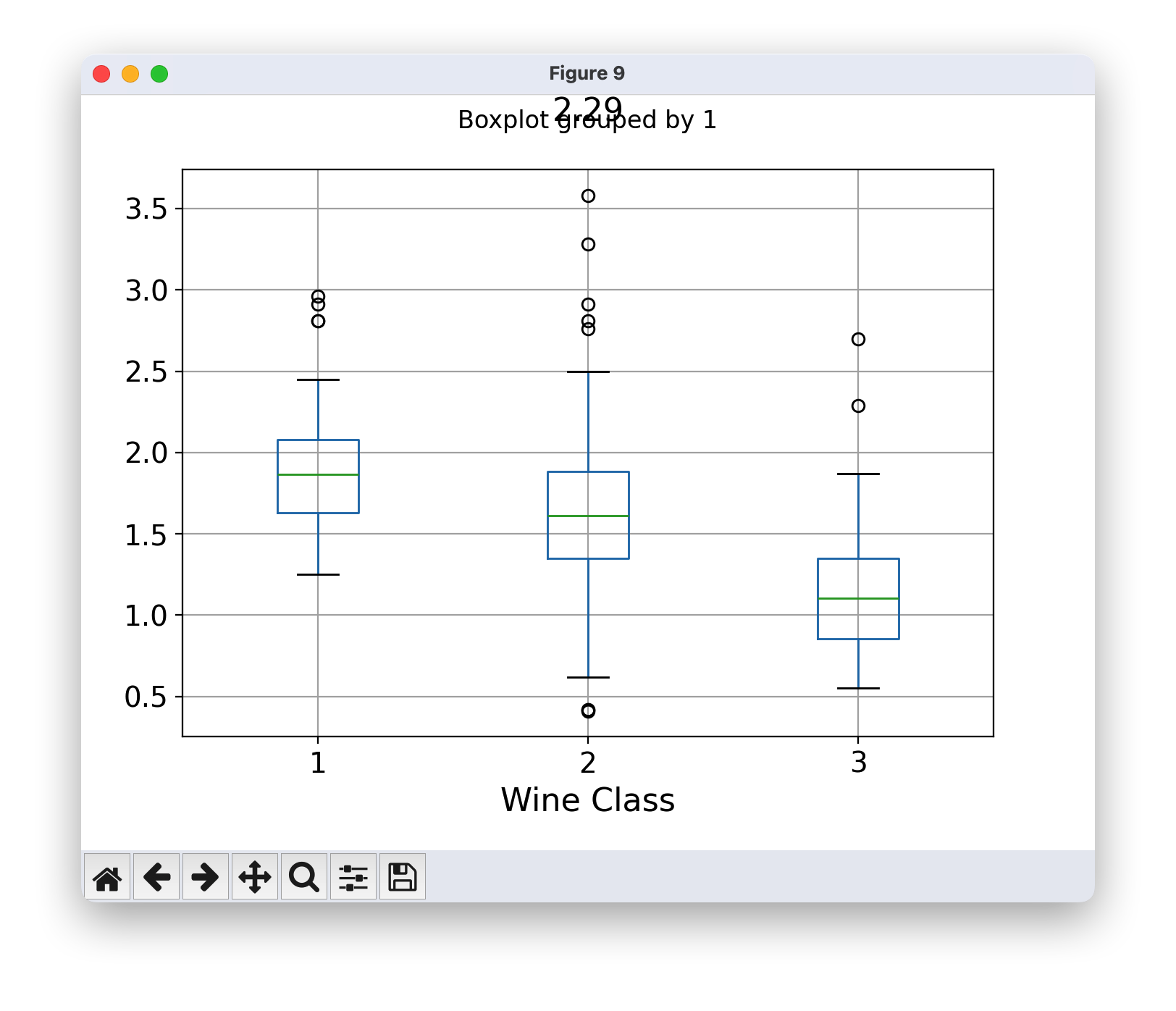
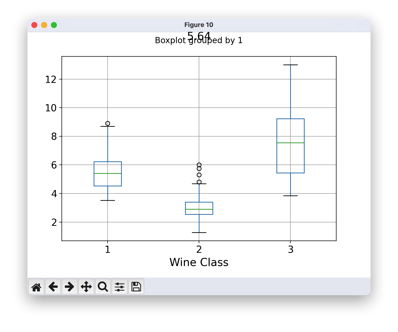
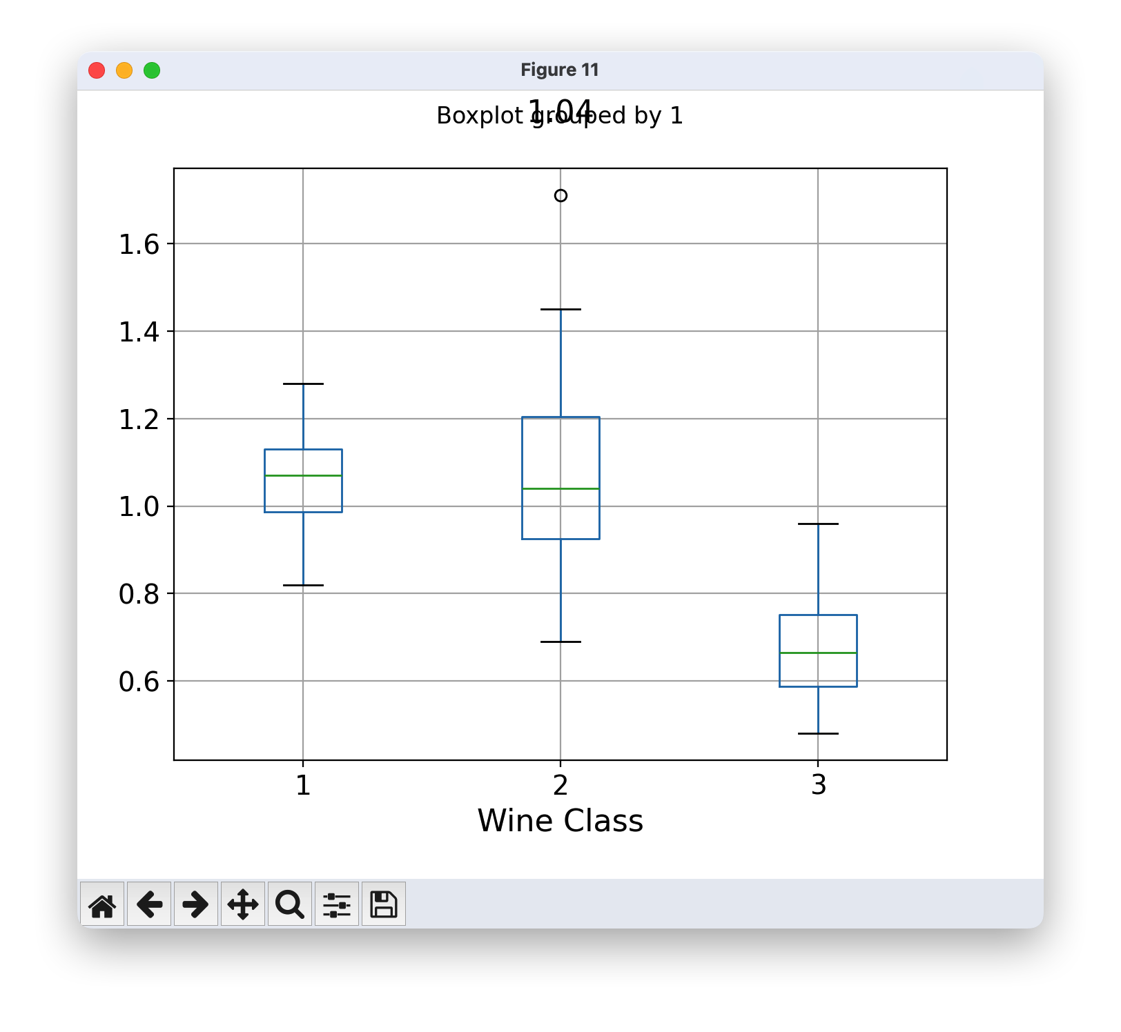
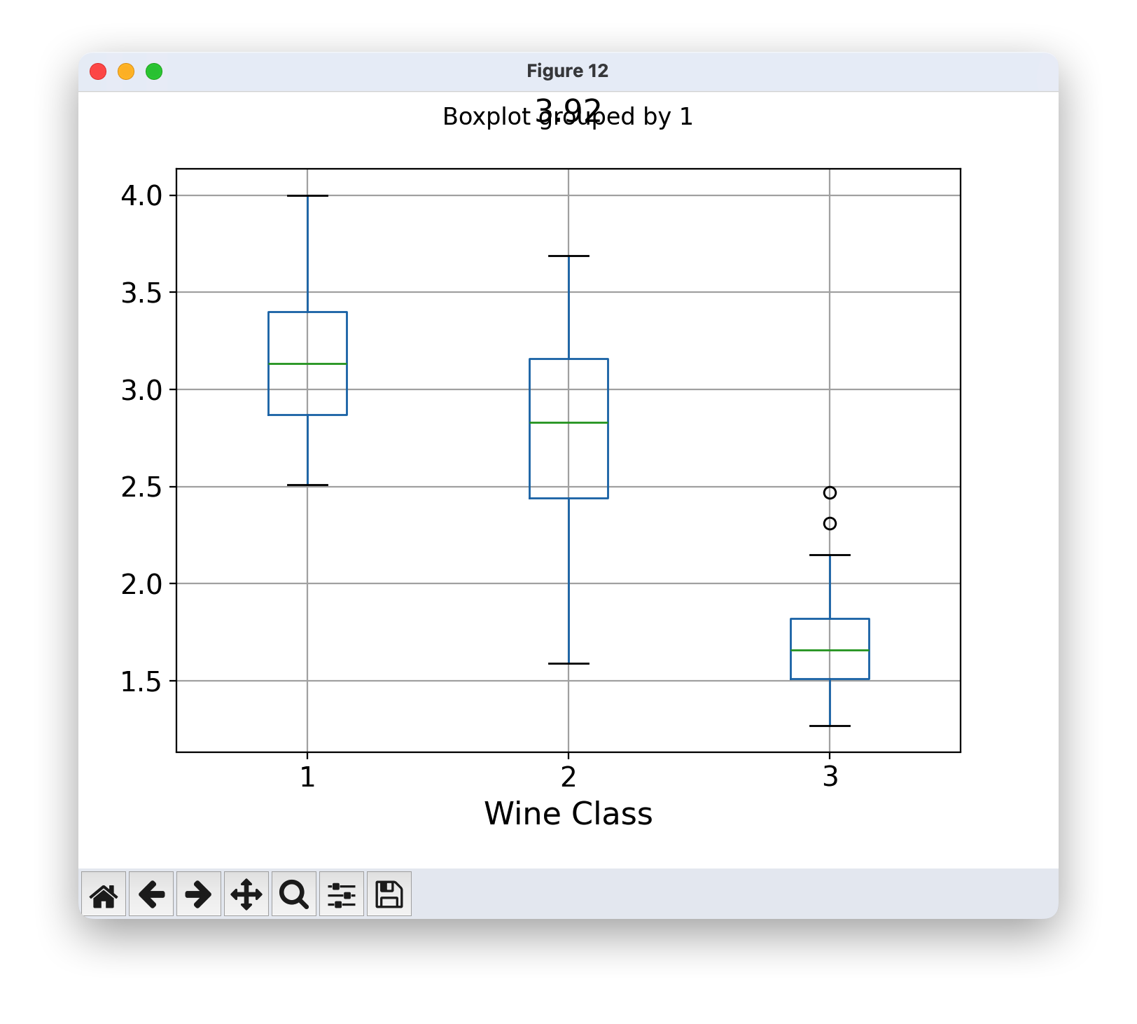
按照输出标签/类别绘制箱形图

for c in df.columns[1:]:
    df.boxplot(c,by='1',figsize=(7,4),fontsize=14)
    plt.title("{}\n".format(c),fontsize=16)
    plt.xlabel("Wine Class", fontsize=16)

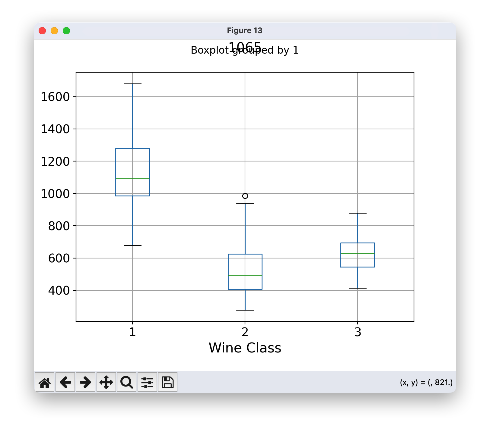
可以看出，某些特征能够相当清晰地对葡萄酒标签进行分类。 例如，碱性度（Alcalinity）、总酚（Total Phenols）或黄酮类化合物（Flavonoids）等特征产生的箱形图具有分离良好的中位数，这些中位数的清晰分离明显地指示了不同的葡萄酒类别。

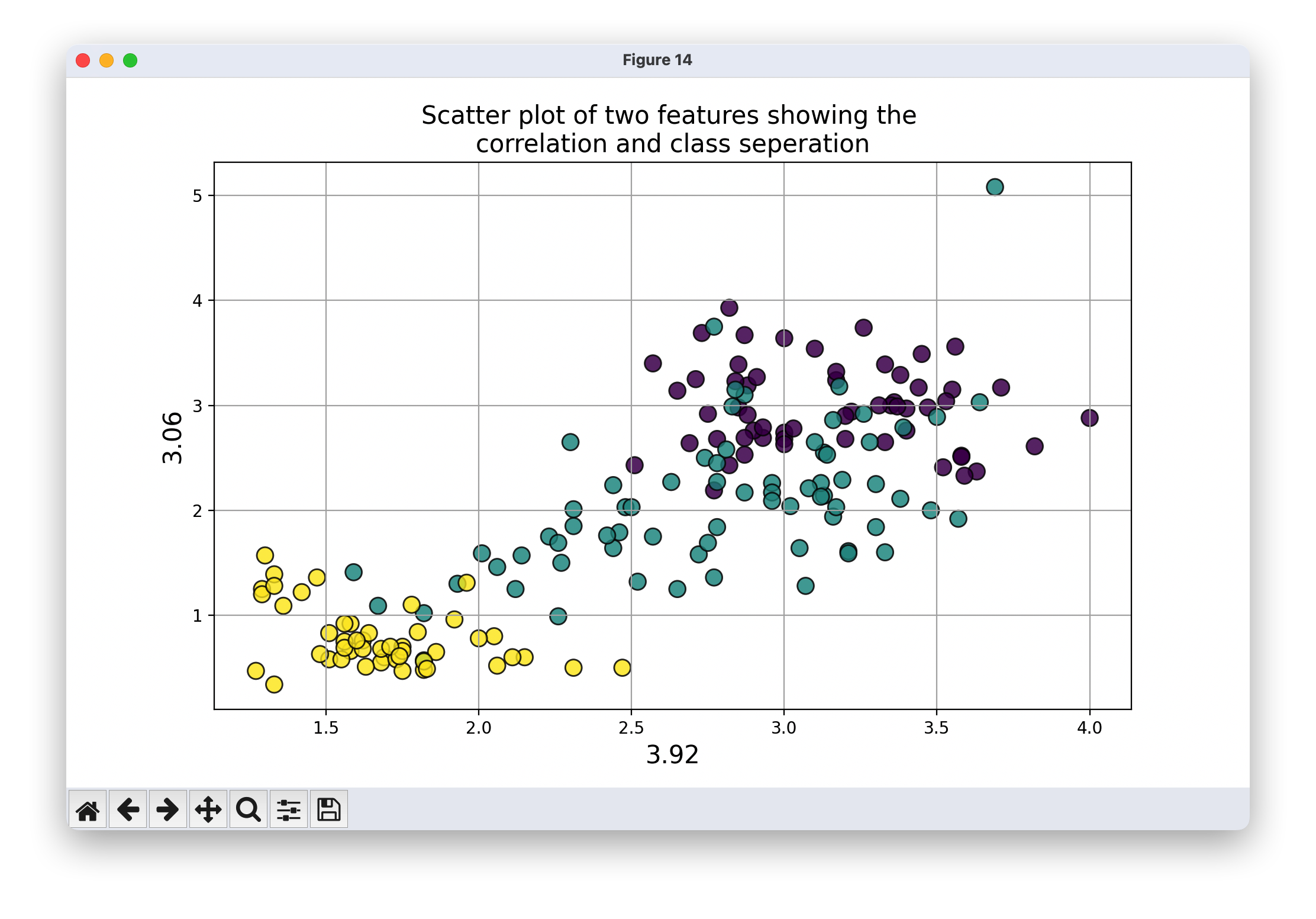
以下是使用两个变量进行类别分离的一个示例

plt.figure(figsize=(10,6))
plt.scatter(df['3.92'],df['3.06'],c=df['1'],edgecolors='k',alpha=0.8,s=100)
plt.grid(True)
plt.title("Scatter plot of two features showing the \ncorrelation and class seperation",fontsize=15)
plt.xlabel("3.92",fontsize=15)
plt.ylabel("3.06",fontsize=15)

特征之间是否独立？绘制协方差矩阵。

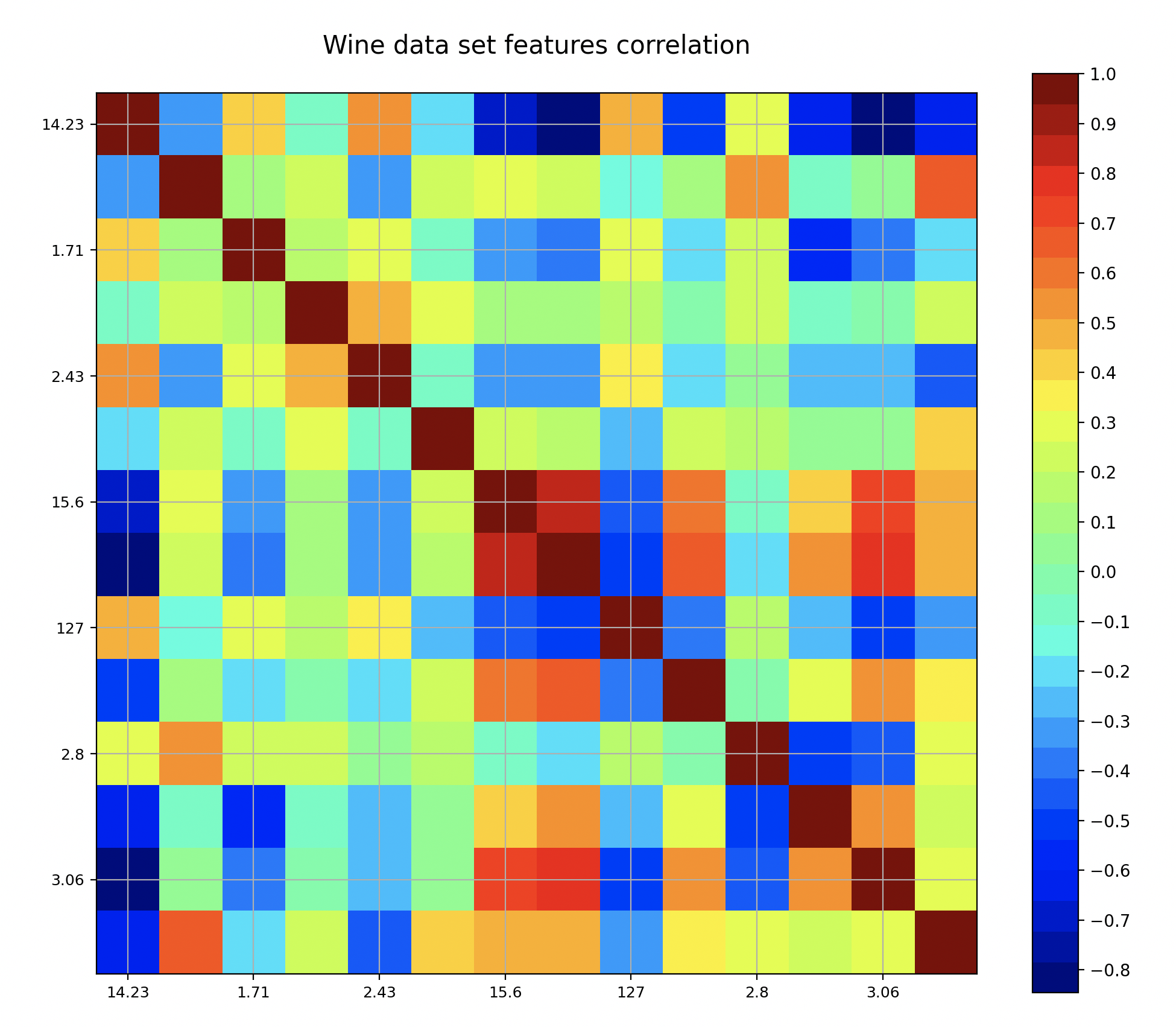
可以看到，特征之间存在一定程度的相关性，也就是说它们并不像朴素贝叶斯（Naive Bayes）技术所假设的那样相互独立。然而，我们仍将应用这个分类器来观察它的性能表现。

def correlation_matrix(df):
    from matplotlib import pyplot as plt
    from matplotlib import cm as cm

    fig = plt.figure(figsize=(16,12))
    ax1 = fig.add_subplot(111)
    cmap = cm.get_cmap('jet', 30)
    cax = ax1.imshow(df.corr(), interpolation="nearest", cmap=cmap)
    ax1.grid(True)
    plt.title('Wine data set features correlation\n',fontsize=15)
    labels=df.columns
    ax1.set_xticklabels(labels,fontsize=9)
    ax1.set_yticklabels(labels,fontsize=9)
    # Add colorbar, make sure to specify tick locations to match desired ticklabels
    fig.colorbar(cax, ticks=[0.1*i for i in range(-11,11)])
    plt.show()

correlation_matrix(df)

1.3朴素贝叶斯分类

测试/训练划分

from sklearn.model_selection import train_test_split

test_size=0.3 # Test-set fraction

X = df.drop('1',axis=1)
y = df['1']
X_train, X_test, y_train, y_test = train_test_split(X, y, test_size=test_size)
X_train.shape
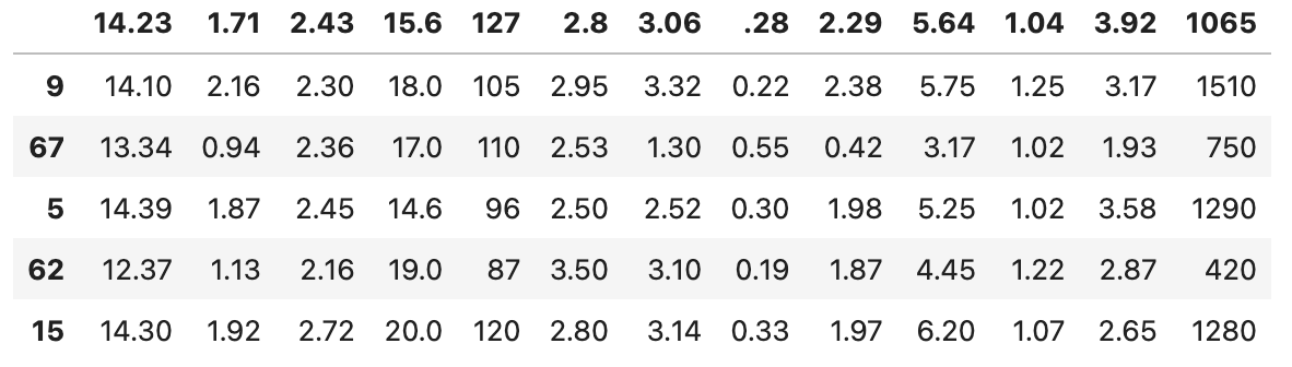
X_train.head()

1.4使用 GaussianNB 进行分类

给定一个类别变量 $y$ 和一组依赖特征向量 $x_1$ 到 $x_n$ ，贝叶斯定理表达了以下关系：

$$P(y\mid x_1,\dots ,x_n)=\frac{P(y)P(x_1,\dots x_n\mid y)}{P(x_1,\dots ,x_n)}$$
使用“特征之间相互独立”的朴素假设
$$P(x_i|y,x_1,\dots ,x_{i-1},x_{i+1},\dots ,x_n)=P(x_i|y),$$
即对于所有的 $i$ ，这个关系可以简化为
$$P(y\mid x_1,\dots ,x_n)=\frac{P(y){\prod }_{i=1}^{n}P(x_i\mid y)}{P(x_1,\dots ,x_n)}$$

由于在给定输入的情况下 $P(x_1,\dots ,x_n)$ 是常数，我们可以使用以下分类规则：
$$P(y\mid x_1,\dots ,x_n)\propto P(y)\prod _{i=1}^{n}P(x_i\mid y)$$
$$\Downarrow$$
$$\hat{y}=\arg \underset{y}{\max }P(y)\prod _{i=1}^{n}P(x_i\mid y),$$
我们可以使用最大后验概率估计来估计 $P(y)$ 和 $P(x_i\mid y)$ ；前者是训练集中类别 $y$ 的相对频率。

GaussianNB () 实现了用于分类的高斯朴素贝叶斯算法。假设特征的似然性服从高斯分布

$$P(x_i\mid y)=\frac{1}{\sqrt{2\pi {\sigma }_y^2}}\exp (-\frac{(x_i-{\mu }_y{)}^2}{2{\sigma }_y^2})$$

参数 ${\sigma }_y$和 ${\mu }_y$ 是使用最大似然估计来估计的。

from sklearn.naive_bayes import GaussianNB
nbc = GaussianNB()
nbc.fit(X_train,y_train)

1.5预测、分类报告和混淆矩阵

y_pred = nbc.predict(X_test)
mislabel = np.sum((y_test!=y_pred))
print("Total number of mislabelled data points from {} test samples is {}".format(len(y_test),mislabel))

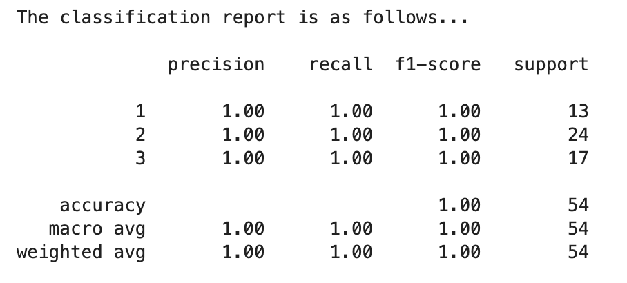
from sklearn.metrics import classification_report
print("The classification report is as follows...\n")
print(classification_report(y_pred,y_test))
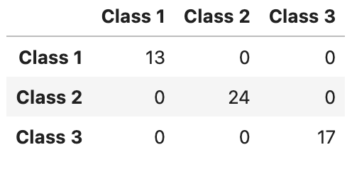
from sklearn.metrics import confusion_matrix
cm = (confusion_matrix(y_test,y_pred))
cmdf = pd.DataFrame(cm,index=['Class 1','Class 2',' Class 3'], columns=['Class 1','Class 2',' Class 3'])
print("The confusion matrix looks like following...\n")
cmdf