案例：用xgboost实现otto商品分类案例

##########################################################################

1、数据准备

1.1 导入数据

import pandas as pd
import numpy as np
import matplotlib.pyplot as plt

1.2 读取数据

1.2.1 用type()命令查看数据的类型，有的时候不同的API要求数据的数据类型不同，随时查看和进行转换

data = pd.read_csv("C:/Python-Project/otto competaion/train.csv")
data.shape
# (61878, 95)

data.head()

1.3 在整体数据中挑选特征和目标数据集

X = data.drop(["id","target"],axis=1)
Y = data["target"]
X.shape,Y.shape
# ((61878, 93), (61878,))

1.4 数据初步可视化

import seaborn as sns
sns.countplot(Y)
plt.show()

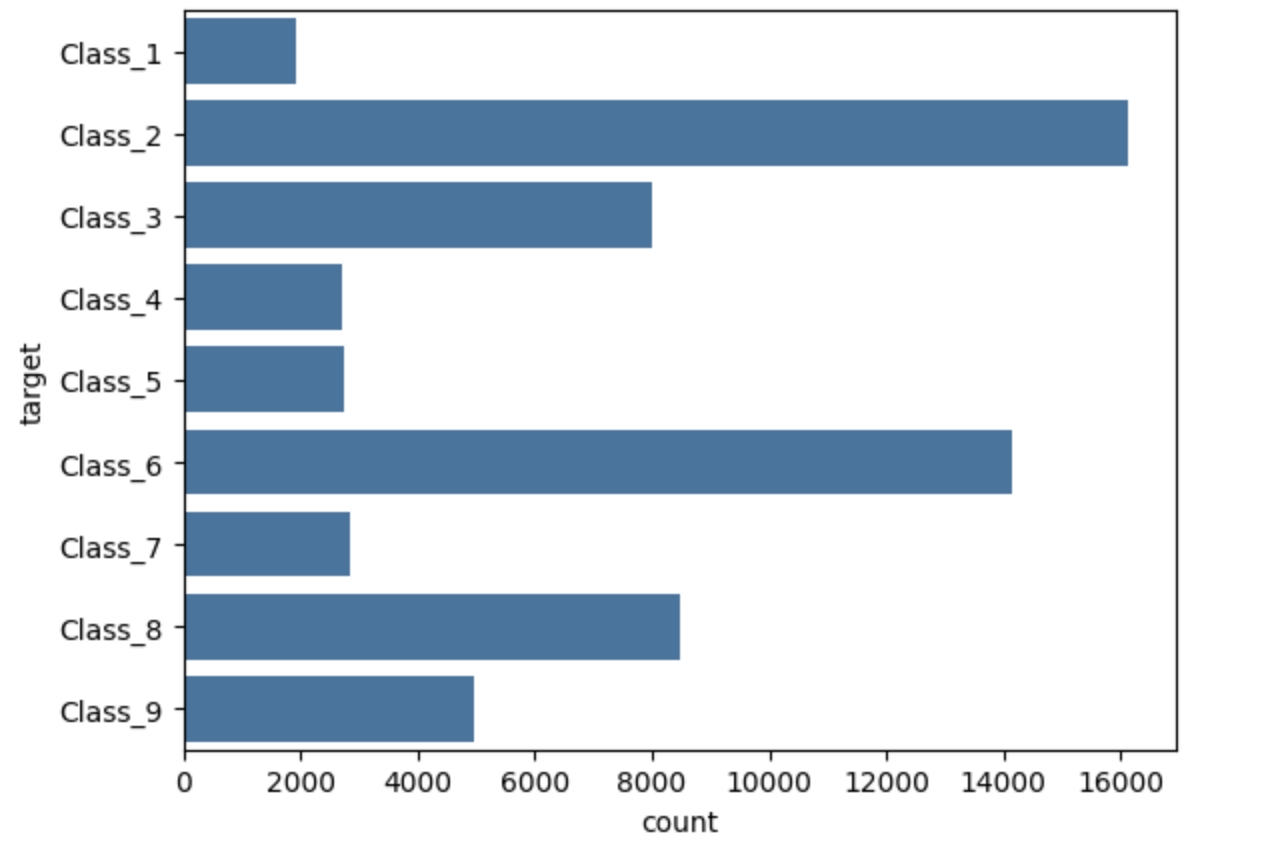
此时目标值数据比较分散，分布不均，为了让算法可以均匀的学到每一个类别的特征，需要对数据进行欠采样处理，处理后的数据会对每个类别的平均抽样

1.5 数据欠采样

from imblearn.under_sampling import RandomUnderSampler
rus = RandomUnderSampler(random_state=0)
x_resampled,y_resampled = rus.fit_resample(X,Y)
x_resampled.shape,y_resampled.shape
# ((17361, 93), (17361,))

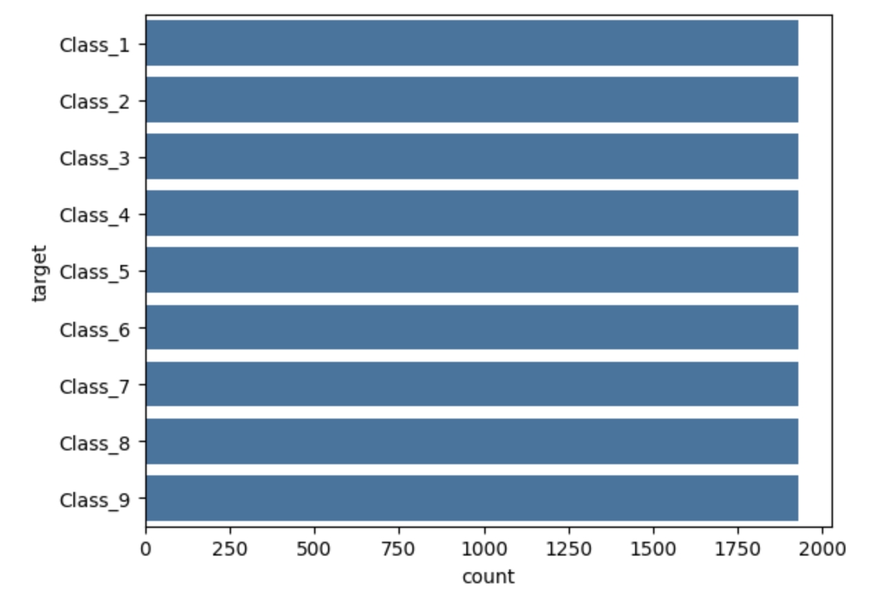
欠采样完毕后，数据总行数变少，但是每个类别都是平均分布的，数据总数为17361，总共9类，则每组数据量为1929

sns.countplot(y_resampled)
plt.show()

1.6 对非数字类特征值进行LabelEncoder处理

from sklearn.preprocessing import LabelEncoder
lb = LabelEncoder()
y_resampled = lb.fit_transform(y_resampled)
y_resampled
# array([0, 0, 0, ..., 8, 8, 8], shape=(17361,))

2、数据预处理

2.1 划分训练集和测试集

案例中选择用StratifiedShuffleSplit代替train_test_split进行数据集的划分

• train_test_split：
  • 适用于数据类别分布相对均匀，或者类别分布对模型性能影响不大的情况。例如，在一些简单的回归问题中，数据没有明显的类别特征，或者在分类问题中类别分布较为均衡时，可以使用 train_test_split。它的优点是简单快速，计算开销小。
• StratifiedShuffleSplit：
  • 主要适用于类别不平衡的分类数据集。在这种数据集中，如果使用 train_test_split 随机划分，可能会导致某个类别在训练集或测试集中的比例与原始数据集差异较大，从而影响模型的训练效果和评估的准确性。而 StratifiedShuffleSplit 能够保证每个类别在训练集和测试集中的比例与原始数据集一致，使得模型在训练和评估时能够更准确地反映不同类别的特征。

 但是上面已经进行了欠采样处理了，这里这一步的有必要吗？

# 用StratifiedShuffleSplit方法来进行训练集和测试集的划分
from sklearn.model_selection import StratifiedShuffleSplit
sss = StratifiedShuffleSplit(n_splits=1,test_size=0.2,random_state=0)
for train_index,test_index in sss.split(x_resampled,y_resampled):
    print(len(train_index))
    print(len(test_index))

    x_train = x_resampled.values[train_index]
    x_test = x_resampled.values[test_index]

    y_train = y_resampled[train_index]
    y_test = y_resampled[test_index]
# 13888
  3473

2.2 数据标准化

from sklearn.preprocessing import StandardScaler
scaler = StandardScaler()
scaler.fit(x_train)
x_train_scaled = scaler.transform(x_train)
x_test_scaled = scaler.transform(x_test)

2.3 PCA降维

from sklearn.decomposition import PCA
pca = PCA(n_components=0.9)
x_train_pca = pca.fit_transform(x_train_scaled)
x_test_pca = pca.transform(x_test_scaled)

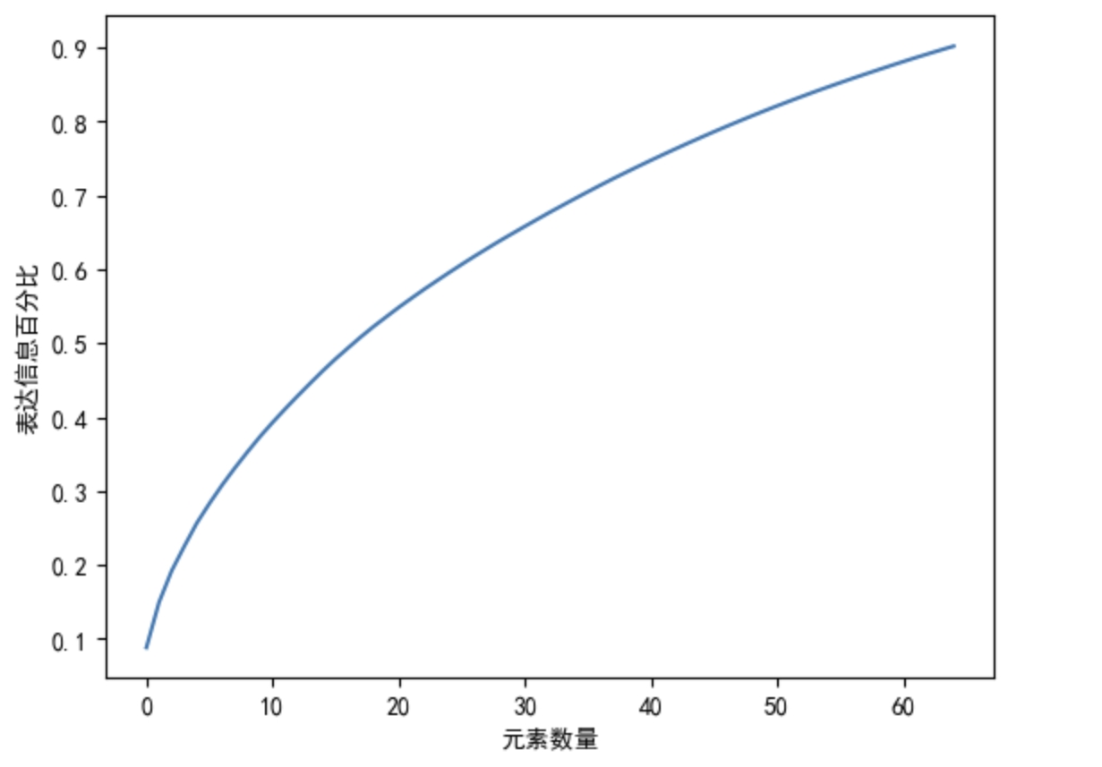
print  shape查看维度，数据从93维降到65维

print(x_train_pca.shape,x_test_pca.shape)
# (13888, 65) (3473, 65)

 主成分累计曲线的作用是显示出元素数量和代表原数据程度的关系

# 显示PCA主成分累计曲线
plt.plot(np.cumsum(pca.explained_variance_ratio_))
plt.xlabel("元素数量")
plt.ylabel("表达信息百分比")
# 设置字体以支持中文显示
plt.rcParams['font.sans-serif'] = ['SimHei']  # 使用黑体字体
# 解决负号显示问题
plt.rcParams['axes.unicode_minus'] = False
plt.show()

3、模型训练

3.1 基本模型训练

from xgboost import XGBClassifier
xgb = XGBClassifier()
xgb.fit(x_train_pca,y_train)

# 输出预测值
y_pre_proba = xgb.predict_proba(x_test_pca)

y_pre_proba
# array([[8.4263504e-01, 3.2945296e-03, 1.2603854e-03, ..., 5.8095489e-02,
        8.7469649e-03, 2.9512435e-02],
       [1.6811924e-02, 1.7416530e-03, 2.2014571e-04, ..., 3.7293904e-04,
        9.7307982e-04, 9.7107983e-01],
       [4.3886024e-04, 7.9340599e-02, 8.8521558e-01, ..., 1.3331524e-02,
        1.8450724e-04, 6.5231987e-05],
       ...,
       [2.0166809e-02, 1.5123079e-04, 2.3353292e-04, ..., 1.9541025e-02,
        9.5690030e-01, 2.9340643e-03],
       [9.8255152e-01, 1.5198133e-03, 1.1549572e-03, ..., 7.2453776e-03,
        3.2669762e-03, 3.5109173e-03],
       [1.0842361e-05, 1.8253126e-04, 1.6896216e-04, ..., 4.8692898e-05,
        9.9796981e-01, 1.1146776e-04]], shape=(3473, 9), dtype=float32)

# logloss评估 
from sklearn.metrics import log_loss
log_loss(y_test,y_pre_proba,normalize=True)
# 0.7375552813900996

到此，初步计算完成了，但是log_loss的值比较高，需要对xgboost中的参数进行优化

3.2 模型调优

3.2.1 n_estimators参数调优

scores_ne = []
n_estimators = [100,200,300,400,500,550,600,700]
for nes in n_estimators:
    print("n_estimators:",nes)
    xgb = XGBClassifier(max_depth = 3,
                        learning_rate = 0.1,
                        n_estimators = nes,
                        objective = "multi:softprob",
                        n_jobs = -1,
                        nthread = 4,
                        min_child_weight = 1,
                        subsample = 1,
                        colsample_bytree = 1,
                        seed = 42)
    xgb.fit(x_train_pca,y_train)
    y_pre = xgb.predict_proba(x_test_pca)
    score = log_loss(y_test,y_pre)
    scores_ne.append(score)
    print("每次测试的log_loss的值是：{}".format(score))
#
n_estimators: 100
每次测试的log_loss的值是：0.7848359172199362
n_estimators: 200
每次测试的log_loss的值是：0.7153972994736512
n_estimators: 300
每次测试的log_loss的值是：0.6908188324177672
n_estimators: 400
每次测试的log_loss的值是：0.6789576854995951
n_estimators: 500
每次测试的log_loss的值是：0.6748054056455964
n_estimators: 550
每次测试的log_loss的值是：0.672917674898804
n_estimators: 600
每次测试的log_loss的值是：0.6723235541249003
n_estimators: 700
每次测试的log_loss的值是：0.6727791973644079

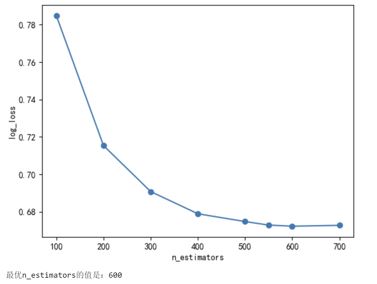
主要思路就是写for in循环，一个一个遍历参数，然后每个参数都看log_loss，选择值最小的那个。

图形化展示log_loss值

plt.plot(n_estimators,scores_ne,"o-")
plt.xlabel("n_estimators")
plt.ylabel("log_loss")
plt.show()
print("最优n_estimators的值是：{}".format(n_estimators[np.argmin(scores_ne)]))

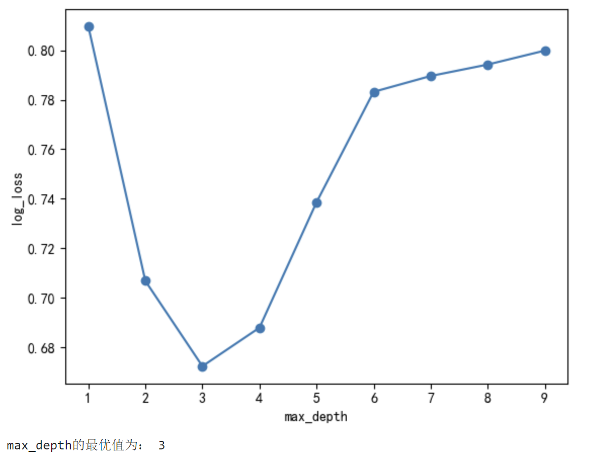
3.2.2 max_depth参数调优

score_md = []
max_depth = [1,2,3,4,5,6,7,8,9]
for md in max_depth:
    print("max_depth的取值为：{}".format(md))
    xgb = XGBClassifier(max_depth = md,
                        learning_rate = 0.1,
                        n_estimators = n_estimators[np.argmin(scores_ne)],
                        objective = "multi:softprob",
                        n_jobs = -1,
                        nthread = 4,
                        min_child_weight = 1,
                        subsample = 1,
                        colsample_bytree = 1,
                        seed = 42)
    xgb.fit(x_train_pca,y_train)
    y_pre = xgb.predict_proba(x_test_pca)
    score = log_loss(y_test,y_pre)
    score_md.append(score)
    print("每次测试的log_loss值是：{}".format(score))
#
max_depth的取值为：1
每次测试的log_loss值是：0.8097415697779353
max_depth的取值为：2
每次测试的log_loss值是：0.7068002259645377
max_depth的取值为：3
每次测试的log_loss值是：0.6723235541249003
max_depth的取值为：4
每次测试的log_loss值是：0.687892772277097
max_depth的取值为：5
每次测试的log_loss值是：0.7385451472328785
max_depth的取值为：6
每次测试的log_loss值是：0.7831879758824114
max_depth的取值为：7
每次测试的log_loss值是：0.7895804582427957
max_depth的取值为：8
每次测试的log_loss值是：0.7942122314471544
max_depth的取值为：9
每次测试的log_loss值是：0.7998475453809357

# 可视化显示
plt.plot(max_depth,score_md,"o-")
plt.xlabel("max_depth")
plt.ylabel("log_loss")
plt.show()
print("max_depth的最优值为：",max_depth[np.argmin(score_md)])

对参数逐一进行调优，最终会得到一组最优参数组合

# 所有参数调优完毕
print("n_estimators的最优解为：{}".format(n_estimators[np.argmin(scores_ne)]))
print("max_depth的最优解为：",max_depth[np.argmin(score_md)])
print("min_child_weight的最优解为：{}".format(min_child_weight[np.argmin(score_mcw)]))
print("subsamples的最优解为:{}".format(subsamples[np.argmin(score_sp)]))
print("colsample_bytree的最优解为：{}".format(colsample_bytree[np.argmin(score_cb)]))
print("learning_rate的最优解为:{}".format(learning_rates[np.argmin(score_lr)]))

#
n_estimators的最优解为：600
max_depth的最优解为： 3
min_child_weight的最优解为：8
subsamples的最优解为:0.7
colsample_bytree的最优解为：0.6
learning_rate的最优解为:0.1

# 最终的模型及参数为
xgb = XGBClassifier(max_depth = 3,
                        learning_rate = 0.1,
                        n_estimators = 600,
                        objective = "multi:softprob",
                        n_jobs = -1,
                        nthread = 4,
                        min_child_weight = 8,
                        subsample = 0.7,
                        colsample_bytree = 1,
                        seed = 42)
xgb.fit(x_train_pca,y_train)
y_pre = xgb.predict_proba(x_test_pca)
print("本次的log_loss值为：{}".format(log_loss(y_test,y_pre)))

本次的log_loss值为：0.6633436401561196

##########################################################################

案例中调优的方法有点麻烦，而且每个参数之间的关联影响也并没有考虑进去。

对于 XGBRegressor（或其他一些模型）fit 之后的 .score 方法，确实是输入 x_test 和 y_test 。这里 x_test 是测试集的特征数据，y_test 是测试集的真实标签，.score 方法会根据模型在 x_test 上的预测结果与 y_test 对比，返回一个评估指标值（如回归中常用的决定系数 R2 ）。

然而，对于 log_loss 函数，它并不需要 x_test ，而是需要 y_test（真实标签）和 y_pre（预测概率） 。log_loss 主要用于评估分类模型预测概率与真实标签之间的差异，所以它关注的是预测概率与真实情况的对比，而非特征数据 x_test 。

总结来说：

• .score 方法：model.score(x_test, y_test)，通过特征数据 x_test 得到预测值，并与真实标签 y_test 对比计算评估指标。
• log_loss 函数：log_loss(y_test, y_pre)，直接对比真实标签 y_test 和预测概率 y_pre 来计算对数损失。